DOI:https://doi-0004.org/6812/17911049866587
Abstract
This study addresses the economic challenges facing Middle East and North Africa (MENA) economies, despite repeated attempts to stabilize the general price level, contain inflation, preserve individuals’ purchasing power, and adopt economic policies and programs consistent with the macroeconomic conditions prevailing during 2001–2022. The study aims to measure the impact of economic growth and inflation on household consumption in a sample of 16 MENA countries, namely Bahrain, Algeria, Egypt, Iran, Iraq, Jordan, Kuwait, Libya, Morocco, the United Arab Emirates, Oman, Qatar, Saudi Arabia, Sudan, Tunisia, and Turkey. To this end, the study applies the Panel ARDL approach using the Pooled Mean Group (PMG) estimator, in addition to Dynamic Common Correlated Effects (DCCE) estimation to account for cross-sectional dependence and cross-country heterogeneity. The findings indicate a dynamic relationship among the variables that differs between the short run and the long run. The PMG results show a positive and statistically significant long-run effect of gross domestic product on household consumption, while inflation has no statistically significant long-run effect. In the short run, both inflation and gross domestic product exert negative and statistically significant effects on household consumption. The causality results also confirm a heterogeneous causal relationship between the independent variables inf and lpib and the dependent variable lcons, with differences in the strength and direction of effects across cross-sectional units. These findings justify the use of econometric models that account for heterogeneity and cross-sectional dependence in panel data analysis.
Keywords: household consumption, economic growth, inflation, Middle East and North Africa, panel data.
Introduction
Climate change and environmental degradation resulting from the unsustainable exploitation of natural resources may lead to successive disruptions in systems that sustain livelihoods across many regions of the world. This means that consumption, as a central component of the current economic model, cannot be viewed separately from sustainability pressures, resource scarcity, and the growing risks generated by conflicts over increasingly limited resources.
The MENA region continues to face broad economic challenges despite its substantial reserves of oil and natural gas. Oil-exporting economies benefited from relatively high energy prices following the lingering effects of the COVID-19 pandemic, as well as the repercussions of the wars in Ukraine and Gaza. Nevertheless, the slowdown in household consumption growth remains a major constraint on economic growth in MENA countries.
According to the International Monetary Fund, restoring price stability, addressing food insecurity, mitigating the cost-of-living crisis, and protecting vulnerable groups have remained key policy priorities in the region. Since 2019, global food commodity prices have increased sharply, reducing the ability of many households to afford basic goods and services after domestic food and energy inflation eroded real income. This situation prompted governments to expand wage increases and subsidies, while also reducing fiscal space for public services and social spending in areas such as health, education, and social protection. Household consumption can therefore be used as an indicator of individual welfare, while also representing a central objective of economic activity.
Based on the above, the main research question can be formulated as follows:
– To what extent do economic growth and inflation affect household consumption in MENA countries during the period 2001–2022?
To answer this main question, the study raises the following sub-questions:
– How can the effects of economic growth and inflation on household consumption in MENA countries be interpreted?
– How do economic stability and improved economic growth affect household consumption in MENA countries?
– Does the nature of the relationship between economic growth, inflation, and household consumption differ between the short run and the long run?
Study hypotheses
Main hypothesis:
There is a statistically significant relationship between economic growth and inflation, on the one hand, and household consumption, on the other hand, in MENA countries during the period 2001–2022.
First sub-hypothesis:
Economic growth significantly affects household consumption in MENA countries, with a possible difference in the direction of the effect between the short run and the long run.
Second sub-hypothesis:
Inflation rates significantly affect household consumption in MENA countries, particularly in the short run through their effect on households’ purchasing power.
Significance of the study
The importance of the study lies in highlighting household consumption as a key determinant of individual welfare, particularly in economies endowed with large natural resources. Many of these economies, especially in the MENA region, have not been able to fully transform resource revenues into sustainable development outcomes. The determinants of consumption are multiple, and most of them affect the relationship between income, consumption expenditure, and macroeconomic stability as reflected by inflation. Household saving is also an important component of aggregate saving because of its connection with consumption on the one hand and private and public investment on the other.
Objectives of the study
– To evaluate the effects of selected economic factors on household consumption.
– To examine the extent to which higher consumption contributes to individual welfare under economic stability and improved economic growth.
– To highlight the role of policies adopted by MENA countries, especially wage increases and subsidy programs.
Previous Studies
Yadiyal (2025), in a study entitled The Relationship Between Inflation and Consumer Spending Patterns, examined the relationship between inflation and consumer spending patterns in India. Using simple regression between inflation and spending and multiple regression over the period 1970–2024, the study included consumer spending, inflation, disposable income, the saving rate, wage growth, and interest rates. The findings indicate a statistically significant negative relationship between inflation and spending, with inflation explaining about 22% of the variation in spending, while the multiple regression model explains more than 94% after adding the accompanying variables.[1]
Burke and Ozdagli (2023) studied the relationship between household inflation expectations and consumer spending behavior. Their study aimed to explain how higher inflation expectations may encourage households to bring consumption forward, particularly for durable goods, in an environment of near-zero nominal interest rates. Using panel data on US households during 2009–2012, the study found that a 1% increase in inflation expectations raises durable goods spending for some groups, while a 1% increase in inflation expectations among all households increases total spending over one quarter by about 1.8% or less. Higher unemployment expectations are also associated with a significant decline in spending across most consumption categories, which limits the stimulative effect of inflation expectations.[2]
Atigala et al. (2022), in a study entitled Driving the Pulse of the Economy or the Dilution Effect: Inflation Impacting Economic Growth, analyzed the effect of inflation on economic growth in Sri Lanka using an ARDL model for the period 2000–2021. The results show a negative relationship between inflation and economic growth in both the short run and the long run. A 1% increase in inflation reduces short-run economic growth by USD 3,427.94 million and long-run economic growth by USD 107,263.8 million, indicating that inflation disrupts growth and that macroeconomic policies require flexibility to stabilize inflation.[3]
Batrancea (2021), in a study entitled Empirical Evidence Regarding the Impact of Economic Growth and Inflation on Economic Sentiment and Household Consumption, provided an econometric analysis of how economic growth and inflation affect the economy and then household consumption. The study focused on the indirect channel through which macroeconomic variables are transmitted to household decisions. Using panel data for several European countries during 2001–2019, the results show that a 1% increase in real economic growth significantly increases the Economic Sentiment Index (ESI), whereas a 1% increase in inflation is associated with a significant deterioration in economic sectors, leading to lower household consumption. Thus, the positive effect of economic growth on consumption exceeds the negative effect of inflation, although inflation remains a constraining factor through declining household confidence.[4]
Lafdal and Dahmani (2020), in their study on the effect of global oil price fluctuations on domestic inflation in the Algerian economy, examined the impact of international oil price fluctuations on the Algerian consumer price index during 1986–2016 using a vector autoregression (VAR) model. The results indicate that oil price changes significantly contribute to inflation in Algeria. Impulse-response functions and shock simulations also show that the price index responds significantly to oil price shocks during the study period.[5]
Živkov, Đurašković, and Manić (2019) examined how oil price changes affect consumer price inflation in eleven Central and Eastern European countries. The study applied a wavelet-based Markov-switching approach to distinguish effects across different time horizons. The findings show that the transmission of oil price changes to inflation is relatively weak in Central and Eastern European countries, since a 100% increase in oil prices is followed by an inflation increase ranging between 1% and 6%.[6]
Abayon, Michael, and Olaronk (2017) studied the consumption function in Nigeria by applying Keynes’ Absolute Income Hypothesis. They used the Granger causality approach to identify long-run and short-run relationships. The dataset consisted of GDP by expenditure type and household consumption expenditure, both at constant 2005 prices, for the period 1970–2011. The results show that the short-run marginal propensity to consume (MPC = 0.78) is lower than the average propensity to consume (APC = 0.88), suggesting a non-proportional and short-run disequilibrium pattern in the Keynesian framework.[7]
Overall, previous studies indicate that elevated inflation, especially when it remains within persistent medium-to-high ranges, reduces household consumption by weakening purchasing power, particularly among lower-income groups, and may also constrain economic growth. Conversely, stable inflation can support consumption by reducing uncertainty and stabilizing household expectations.
Study Outline
– Consumption under fluctuations in economic factors
– Econometric study of the impact of economic growth and inflation on household consumption in MENA countries
1. Consumption under fluctuations in economic factors
Household consumption is one of the main objectives of economic activity. Excessive consumption behavior increases domestic consumer demand and may lead to higher inflationary pressures, which represent risks for individuals, the economy, currencies, and markets. Inflation weakens citizens’ purchasing power and leads to price jumps. For this reason, household consumption plays an important role in economic growth, which requires identifying its economic and social determinants and examining the role of customs and traditions in either increasing or reducing consumption.[8]
The current expenditure of households on goods and services is referred to as household consumption, while the part of income that is not used for consumption is referred to as saving.[9]
According to the modern concept of consumption, consumption refers to the utility derived from spending on economic goods. It includes private consumption, which corresponds to the household sector, and public consumption, which corresponds to the government sector.[10]
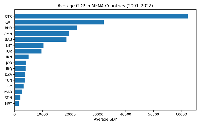
Figure (01): Average GDP in MENA Countries (2001–2022)
Source: Author’s calculations based on World Bank data.
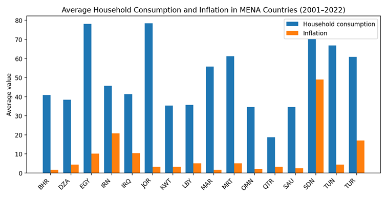
Figure (02): Average Household Consumption and Inflation in MENA Countries (2001–2022)
Source: Author’s calculations based on World Bank data.
Figure (01) shows that Qatar recorded the highest average GDP during 2001–2022, reaching 62,216.3, followed by Kuwait with 32,133.99. By contrast, Mauritania recorded the lowest average in the sample, while Egypt recorded an average of 3,237.01 during the same period. According to Figure (02), household consumption recorded the highest averages in Jordan at 78.42, Egypt at 78.12, and Sudan at 70.27 during 2001–2022. Inflation reached its highest average in Sudan at 49.03%, followed by Iran at 20.75% and Iraq at 10.39%, while Bahrain registered the lowest average inflation rate at 1.65% during the same period.
2. Econometric study of the impact of economic growth and inflation on household consumption in MENA countries
The relationship between economic variables and household consumption has taken different directions in both theory and empirical research. This section measures the impact of economic growth and inflation on household consumption in MENA countries. Based on the previous studies, the model is specified with gross domestic product and inflation as independent variables, while household consumption is the dependent variable. The analysis covers the period 2001–2022 for 16 MENA countries, namely Bahrain, Algeria, Egypt, Iran, Iraq, Jordan, Kuwait, Libya, Morocco, the United Arab Emirates, Oman, Qatar, Saudi Arabia, Sudan, Tunisia, and Turkey. The data were obtained from the World Bank and the Organization of Arab Petroleum Exporting Countries (OAPEC). Some outlying observations were adjusted using statistical procedures, and the model was specified as follows:
lconsᵢₜ = α₀ + α₁ lpibᵢₜ + α₂ infᵢₜ + μᵢ + εᵢₜ
– lconsᵢₜ represents household consumption in country i during period t
– lpibᵢₜ represents gross domestic product in country i during period t
– infᵢₜ represents inflation in country i during period t
– εᵢₜ represents the error term
Model specification:
Table (01): Model specification
| Lcons | Lpib | INF | |
| Obs | 352 | 352 | 352 |
| Mean | 3.83 | 8.88 | 5.94 |
| Std. Dev. | 0.41 | 1.02 | 5.48 |
| Minimum | 2.59 | 7.10 | 0.30 |
| Maximum | 4.5 | 11.20 | 17.34 |
Source: EViews 10 output.
The table shows that the mean value of household consumption reached 3.83 during 2001–2022, while the mean values of the independent variables ranged between 8.88 and 5.94. The standard deviation of household consumption reached 0.41 during the same period, whereas the standard deviations of the explanatory variables ranged between 1.02 and 5.48. Overall, the descriptive statistics show a reasonable degree of homogeneity among the observations.
Correlation matrix
Table (02): Correlation matrix
| Lcons | Lpib | INF | |
| Lcons | 1 | ||
| Lpib | -0.73 | 1 | |
| INF | 0.21 | -0.29 | 1 |
Source: Stata 17 output.
The table indicates weak correlations among most variables. The correlation between inflation and household consumption reached 0.217, while the correlation between inflation and GDP reached -0.291. The relationship between GDP and household consumption recorded a relatively strong inverse correlation of -0.736, or about 73.6%.[11]
2.1 Dependence and homogeneity tests
Slope homogeneity test:
To verify slope homogeneity across the individuals in the sample, namely MENA countries, the Pesaran and Yamagata (2008) test is used. The following table presents the results.
Table (03): Results of the slope homogeneity test
| Delta | p-value | |
| Δ | 9.29 | 0.000 |
| Δadj | 10.27 | 0.000 |
Source: Stata 17 output.
The results indicate that the null hypothesis of homogeneous slope coefficients is rejected at the 5% significance level, based on the Delta and adjusted Delta statistics and their probability values. Accordingly, heterogeneity exists across the study variables, which supports the use of heterogeneous panel methods in which slope parameters may differ across cross-sectional units.
Cross-sectional dependence test:
Table (04): Cross-sectional dependence test results
| Variable | CD-test | p-value |
| lcons | 14.52 | 0.00 |
| lpib | 12.95 | 0.00 |
| inf | 9.27 | 0.00 |
| Pesaran CD test | 15.22 | 0.0000 |
Source: Stata 17 output.
The table shows that the probability value of the CD test is below 5%, indicating the presence of cross-sectional dependence among the countries.[12]
2.3 Estimation of the model using static panel data models
Panel data methods are used to estimate the relationship under study through the Fixed Effects Model (FEM) and the Random Effects Model (REM). Stata 17 was used to estimate the model and obtain the following results:
Table (05): Model estimation (fixed effects and random effects)
| Dependent variable: household consumption | ||
| Period: 2001–2022 N = 16 T = 21 Total panel observations: 352 | ||
| Variables | Fixed Effects Model | Random Effects Model |
| lpib | -0.240 (0.0627) | -0.270 (0.0439) |
| inf | -0.00657 (0.00229) | -0.00632 (0.00227) |
| Constant | 6.003 (0.557) | 6.264 (0.396) |
| Observations | 352 | 352 |
| R-squared | 0.062 | |
| Number of crossid | 16 | 16 |
Source: Stata 17 output.
The table shows that most individual and joint probability values in the FEM and REM models are below 0.05, indicating statistical significance. The coefficients of the explanatory variables are negative in both models. The GDP coefficient reached -0.240 in the fixed effects model and -0.270 in the random effects model, while the inflation coefficient reached -0.00657 and -0.00632 respectively. This indicates a negative and statistically significant effect of both variables on household consumption within the static panel models.
2.3.2 Model selection between Fixed Effects and Random Effects
To determine which of the two models is more appropriate, the Hausman test is used to identify the specification that is more suitable for estimating the model. The following table presents the obtained results:
Table (06): Model selection between Fixed Effects and Random Effects
| Hausman test | |
| chi2(4) | Prob |
| 0.95 | 0.62 |
Source: Stata 17 output.
The probability value of the Hausman test is 0.62, which is greater than 0.05. Thus, the alternative hypothesis H₁ is rejected, and the null hypothesis of no systematic difference between the estimators is accepted. Accordingly, the Random Effects Model is considered the appropriate specification for analyzing the relationship among the study variables in the group of MENA countries.
Based on the model selection results, and since the Random Effects Model is the preferred specification for estimating the effect of GDP and inflation on household consumption in MENA countries during 2001–2022, the model is written as follows:
lcons = 6.26 – 0.27 lpib – 0.006 inf
Analysis of Random Effects estimation results
Based on the Random Effects estimation results, the coefficient of determination R² is about 6.2%. This indicates that the model explains a limited share of the changes in household consumption, while a substantial share of the variation remains associated with other factors not included in the model. The constant term is positive and statistically significant, reflecting a baseline level of household consumption that differs across the countries in the sample.
The estimated coefficients of the explanatory variables are statistically significant. The GDP coefficient in the Random Effects Model is -0.270, meaning that a one-unit increase in GDP is associated with a decline in household consumption of about 0.270 units in the logarithmic specification. The inflation coefficient is -0.00632, indicating that a one-unit increase in inflation reduces household consumption by about 0.00632 units, ceteris paribus.
This analysis clarifies the nature of the relationship between the dependent variable and the independent variables. There is an inverse relationship between GDP and inflation, on the one hand, and household consumption, on the other hand. Economically, this result reflects the effect of inflationary pressures and changes in economic activity on households’ consumption capacity within the static model.
Since the Hausman test supports the Random Effects Model, the variation in the effects of GDP and inflation on household consumption across MENA countries is captured through the country-specific random component of the model.
2.4 Estimation of the model using dynamic panel data
2.4.1 Stationarity analysis of the model variables
Stationarity testing for cross-sectional time series data relies on widely used first- and second-generation unit root tests, including LLC, IPS, and Fisher-ADF tests. These tests aim to identify the time-series properties of the variables included in the panel model. Given the evidence of parameter heterogeneity and cross-sectional dependence, second-generation tests, particularly the CIPS test, are also applied to each variable separately. The results are reported in the following table:
Table (07): Panel unit root test results
| Variables | At level | At level | At first difference | At first difference |
| CIPS | Critical value | CIPS | Critical value | |
| lcons | -2.04 | -2.15 | -4.39 | -2.15 |
| lpib | -1.28 | -2.15 | -3.53 | -2.15 |
| inf | -2.33 | -2.07 |
Source: Stata 17 output.
The table shows that household consumption lcons and GDP lpib are non-stationary at level but become stationary after taking first differences, which means that both variables are integrated of order one I(1). By contrast, the inflation series inf is stationary at level, meaning that it is integrated of order zero I(0).
2.4.2 Cointegration test for the study variables
After conducting the stationarity tests and finding that the variables have mixed orders of integration, the analysis proceeds to test for long-run cointegration relationships among the variables using the Pedroni panel cointegration test.
The Pedroni test is one of the most widely used tests for detecting cointegration among variables in panel data. Pedroni proposed seven statistics for testing the possibility of cointegration in long panels. These statistics are classified into within-dimension and between-dimension statistics, and they approximately follow the standard normal distribution.[13]
Table (08): Cointegration test results
| Test statistic | Panel | Group |
| V | -0.96 | 0.00 |
| Rho | 1.08 | 2.38 |
| T | -1.29 | -0.70 |
| ADF | 1.67 | 1.50 |
Source: Stata 17 output.
The results indicate that most Pedroni statistics support the presence of cointegration, except for some statistics that do not show sufficient significance. Therefore, the alternative hypothesis of a long-run equilibrium relationship among household consumption, GDP, and inflation is accepted, which justifies moving to Panel ARDL estimation.
2.5 Selection of the appropriate dynamic panel model (estimation using PMG, MG, and DFE)
After examining the order of integration of the explanatory variables and the dependent variable, the Panel ARDL model is estimated using the Mean Group (MG), Pooled Mean Group (PMG), and Dynamic Fixed Effects (DFE) estimators. The Hausman test is used to compare these estimators, and the results are presented in the following tables:[14]
Table (09): Estimation results using PMG, MG, and DFE
| Variables | Long run | |||||
| PMG | MG | DFE | ||||
| Coefficient | t-Student | Coefficient | t-Student | Coefficient | t-Student | |
| inf | 0.00 | 0.88 | -0.01 | -1.35 | 0.00 | 0.83 |
| lpib | 0.41 | 9.32 | 0.24 | 0.82 | -0.16 | -1.07 |
| Variables | Short run | |||||
| PMG | MG | DFE | ||||
| Coefficient | t-Student | Coefficient | t-Student | Coefficient | t-Student | |
| ECT | -0.25 | -6.70 | -0.38 | -7.44 | -0.28 | -8.14 |
| d.inf | -0.00 | -3.30 | -0.00 | -2.52 | -0.00 | -4.73 |
| d.lpib | -0.76 | -5.32 | -0.64 | -3.71 | -0.75 | -10.45 |
| c | 0.05 | 1.09 | 1.71 | 1.67 | 1.51 | 3.47 |
Source: Stata 17 output.
Table (10): Model selection tests for the appropriate Panel ARDL specification
| Hausman test | Hausman test | ||
| MG vs PMG | Prob | PMG vs DFE | Prob |
| 3.09 | 0.21 | 0.73 | 0.69 |
Source: Stata 17 output.
The Hausman test comparing the MG and PMG estimators shows a probability value of 0.2137, which is greater than 0.05. Therefore, the null hypothesis supporting the suitability of the PMG estimator is not rejected. Similarly, the comparison between PMG and DFE shows a probability value of 0.6943, which also exceeds 0.05. This strengthens the choice of PMG as the more appropriate estimator for the dynamic relationship among the study variables.
Based on the comparison among the three estimators, the Pooled Mean Group estimator within the Panel ARDL framework is adopted as the most appropriate specification for estimating the relationship between GDP, inflation, and household consumption in MENA countries.
2.5.1 Analysis of ARDL/PMG estimation results
The dynamic estimation results using DFE, MG, and PMG indicate the existence of a long-run equilibrium relationship between the dependent variable and the independent variables. This is confirmed by the negative and statistically significant error correction term ECT in all three models. The ECT reached -0.286 in the DFE model, -0.384 in the MG model, and -0.258 in the PMG model, implying that about 25.8% to 38.4% of short-run disequilibrium is corrected within one period toward the long-run equilibrium.
Long run: Inflation inf has no statistically significant effect in the models, as the t-Student values remain below the accepted thresholds of statistical significance. Economically, this may reflect the role of subsidies and price-control policies in reducing the transmission of inflation to household expenditure. In contrast, GDP lpib has a positive and statistically significant effect in the PMG model, with a coefficient of 0.41 and a t-statistic of 9.32. This means that a 1% increase in lpib raises household consumption by about 0.41% in the long run, reflecting the role of higher GDP in strengthening households’ income capacity and supporting consumption growth over time.
Short run: The results show that the first differences of inflation and GDP have negative and statistically significant effects in the three models. The coefficients of d.inf and d.lpib are negative, and their t-Student values are statistically significant. This indicates that short-run shocks in inflation and GDP temporarily reduce household consumption before it gradually returns to its long-run equilibrium path.
Estimation using DCCE (Dynamic Common Correlated Effects)
Table (11): DCCE estimation results
| Variables | Long run |
| inf | 0.00282 (0.00976) |
| lpib | -0.203 (0.286) |
| Variables | Short run |
| ECT | -0.291 (0.130) |
| d.inf | -0.00613 (0.00213) |
| d.lpib | -0.711 (0.145) |
| R-squared | 0.479 |
| CD | 10.22 (0.00) |
Source: Stata 17 output.
After applying the DCCE estimator, the results show that the CD test statistic is 10.22 with a probability value of 0.00, confirming statistically significant cross-sectional dependence across the countries in the sample. This justifies the use of estimators that account for cross-sectional dependence alongside cross-sectional heterogeneity. The error correction term is negative and statistically significant, with ECT = -0.291, indicating the existence of a long-run equilibrium relationship among the study variables. This means that about 29.1% of short-run disequilibrium is corrected in each period toward the long-run equilibrium.[15]
The long-run estimates show that the inflation and GDP coefficients are not statistically significant. The inflation coefficient is 0.00282 with a standard error of 0.00976, while the GDP coefficient is -0.203 with a standard error of 0.286. This means that these two variables do not exert a statistically significant long-run effect on household consumption under the DCCE estimator. Economically, this may be explained by structural factors that limit the transmission of inflation and GDP changes to consumption behavior, such as government subsidies, price-control policies, income heterogeneity, differences between oil and non-oil economies, and the dependence of consumption in some countries on transfers and public spending rather than real output.
In the short run, the results show that GDP has a negative and statistically significant effect, with the coefficient of d.lpib reaching about -0.711. Inflation is also negative and statistically significant, with a coefficient of -0.00613, although its magnitude is smaller than that of GDP. This indicates that short-run shocks in GDP and inflation temporarily reduce household consumption.
The R-squared value of 0.479 indicates that the model explains about 47.9% of the variation in household consumption, which is a meaningful explanatory capacity in a panel data setting, especially given the structural differences across MENA countries.
Comparison between PMG and DCCE
Table (12): Comparison between PMG and DCCE
| Long run | ||||
| xtpmg–MG | xtdcce2–MG | xtdcce2–MG-t | xtdcce2–CCE | |
| inf | 0.00239 (0.00272) | 0.00282 (0.00976) | 0.000819 (0.00211) | 0.0134 (0.0789) |
| lpib | 0.414 (0.0444) | -0.203 (0.286) | -0.0589 (0.110) | -0.180 (2.091) |
| Short run | ||||
| xtpmg–MG | xtdcce2–MG | xtdcce2–MG | xtdcce2–CCE | |
| ec | -0.258 (0.0385) | -0.291* (0.130) | -0.291 (0.0553) | -0.117 (1.308) |
| d.inf | -0.00644 (0.00195) | -0.00613 (0.00213) | -0.00613 (0.00213) | -0.00332 (0.00184) |
| d.lpib | -0.768 (0.144) | -0.711 (0.145) | -0.711 (0.145) | -0.522 (0.0916) |
| Cons | 0.0593 (0.0543) | |||
| cd | 10.22 | 10.22 | 0.125 | |
| cdp | 0 | 0 | 0.900 | |
Source: Stata 17 output.
The comparison between PMG and DCCE reveals clear differences in the estimation of long-run and short-run relationships. In the long run, inflation has no statistically significant effect in all models. GDP lpib has a positive and statistically significant effect only under the PMG estimator, with a coefficient of 0.414 and a standard error of 0.0444. This indicates that a 1% increase in lpib is associated with an increase in household consumption of about 0.41% in the long run. The other DCCE specifications, namely MG, MG-t, and CCE, do not show a statistically significant long-run effect, since the lpib coefficients are either negative, weak, or statistically insignificant.[16]
In the short run, the error correction term ec confirms the presence of a long-run equilibrium relationship, as it is negative and significant in the PMG model at -0.258 and in the DCCE-MG model at -0.291. This means that the speed of adjustment ranges between 25.8% and 29.1% within one period. However, the coefficient loses significance in the DCCE-CCE specification. The results also show that d.lpib has a negative and statistically significant effect in the different models, with coefficients ranging between -0.768 and -0.522. Inflation also shows a negative short-run effect, but its magnitude is smaller than that of GDP.
The Pesaran CD test indicates that cross-sectional dependence persists in the DCCE-MG and DCCE-MG-t specifications, where the test statistic reaches 10.22 with a probability value of 0.000. In contrast, the statistic falls to 0.125 with a probability value of 0.900 under the DCCE-CCE specification. This means that the CCE specification is more able to address cross-sectional dependence, although its long-run estimates differ from those obtained using PMG.
Table (13): Hausman test
| hausman MG pooled, sigmamore | hausman PMG pooled, sigmamore | ||
| chi2(5) | Prob | chi2(5) | Prob |
| 1.43 | 0.9205 | 1.98 | 0.8519 |
Source: Stata 17 output.
Since the Hausman probability values exceed the 5% significance level, reaching 0.9205 in the comparison between MG and the pooled model and 0.8519 in the comparison between PMG and the pooled model, the null hypothesis is not rejected. This indicates that there are no systematic differences among the estimators under comparison. Based on the previous comparison between MG, PMG, and DFE, the PMG estimator can be adopted as the most appropriate specification in this study. The PMG estimator imposes long-run homogeneity across countries while allowing short-run coefficients, error-correction terms, and error variances to differ across cross-sectional units.
2.5.2 Diagnostic tests for model adequacy
LM and Wald tests for heteroscedasticity
Table (14): LM and Wald test results
| Panel data Heteroscedasticity Breusch-Pagan (LM) Test | ||
| Test | Statistic | p-value |
| Lagrange Multiplier Test | 75.96 | 0.00 |
| Panel Data Heteroscedasticity Wald Test | ||
| Wald Test | 15.73 | 0.00 |
Source: Stata 17 output.
The table shows that the probability values of both the Breusch-Pagan LM test and the Wald test are below the 5% significance level, reaching 0.0000 and 0.0001 respectively. This leads to the rejection of the null hypothesis of homoscedasticity and confirms the presence of heteroscedasticity in the model.
Multicollinearity and serial correlation
Table (15): VIF and Wooldridge test results
| Variance Inflation Factor (VIF) test | ||
| Variable | VIF | 1/VIF |
| inf | 1.09 | 0.91 |
| lpib | 1.09 | 0.91 |
| Mean VIF | 1.09 | |
| Wooldridge test | ||
| Test | Statistic | p-value |
| Wooldridge test | 8.88 | 0.009 |
Source: Stata 17 output.
The VIF test shows that the VIF values for inflation and GDP are both 1.09, which is below the commonly accepted threshold of 10. This indicates the absence of multicollinearity among the independent variables. The Wooldridge test for autocorrelation in panel data has a probability value of 0.0093, which is below the 10% significance level. Therefore, the null hypothesis of no serial correlation is rejected, confirming the presence of autocorrelation in the model.[17]
2.6 Causality test for heterogeneous panel data
The Granger non-causality test developed by Dumitrescu and Hurlin (2012) accounts for heterogeneity in panel data by estimating separate causal relationships for each cross-sectional unit. This allows the test to capture differences in the direction of causality across the countries under study. The null hypothesis assumes no Granger causality in all cross-sectional units, while the alternative hypothesis assumes heterogeneous causality in at least one cross-sectional unit. The results of this test are presented in the following table.[18]
Table (16): Granger causality test for heterogeneous panel data
| Dumitrescu and Hurlin (2012) causality test | ||
| Test | Statistic | p-value |
| W-bar | 3.2921 | |
| Z-bar | 6.4829 | 0.0000 |
| Z-bar tilde | 4.9443 | 0.0004 |
| Juodis, Karavias and Sarafidis (2021) causality test | ||
| HPJ Wald test | 3.3477 | 0.0673 |
Source: Stata 17 output.
The results show a heterogeneous causal relationship among the study variables at the panel level. The W-bar statistic is 3.2921, the Z-bar statistic is 6.4829 with a probability value of 0.0000, and the Z-bar tilde statistic is 4.9443 with a probability value of 0.0004. These results lead to the rejection of the null hypothesis of non-causality and support the existence of statistically significant causality in at least some cross-sectional units. This reflects the heterogeneity of causal directions among the countries in the sample.
Economically, GDP affects consumption through income, employment, public expenditure, and overall economic activity. Improved economic activity in countries with broader productive bases can strengthen households’ spending capacity, while the same effect may not appear in rentier economies where consumption is more closely linked to subsidies and transfers than to real production. Inflation affects household consumption through the purchasing-power channel, since higher prices reduce households’ real income and push them to reallocate spending toward essential goods while reducing spending on non-essential or durable goods. The heterogeneity of causality reflects differences in subsidy systems, income levels, consumption structures, and wage flexibility across MENA countries.
The Juodis, Karavias and Sarafidis test reports an HPJ Wald statistic of 3.3477 with a probability value of 0.0673, which is statistically significant only at the 10% level. This provides weaker additional support for dynamic causality after accounting for cross-sectional dependence and common factors. Overall, the results indicate that the independent variables inf and lpib help explain changes in household consumption in some cross-sectional units, with differences in the strength and direction of effects across countries. This further justifies the use of econometric models that account for heterogeneity and cross-sectional dependence.[19]
Conclusion
Despite the substantial natural resource endowments of MENA countries, high dependence on oil resources has made many of these economies more vulnerable to oil price fluctuations, with implications for GDP, income, and household consumption. Attempts to control the general price level and inflation have aimed to preserve individuals’ purchasing power and reduce pressures on consumption and saving behavior. During 2001–2022, the highest inflation rates were recorded in Sudan and Iran. GDP data show that Qatar and Kuwait achieved the highest levels, while household consumption recorded its highest averages in Jordan and Egypt.
The study applied the Panel ARDL methodology using the PMG estimator, together with DCCE estimations that account for cross-sectional dependence and heterogeneity across the sample countries. The results show that the nature of the effect differs between the short run and the long run. In the long run, the PMG model shows a positive and statistically significant effect of GDP on household consumption, while inflation has no statistically significant effect. In the short run, shocks to both GDP and inflation are negative and statistically significant, with a negative and significant error correction term confirming the adjustment mechanism toward long-run equilibrium.
The main findings of the study can be summarized as follows:
– Economic growth remains weak in several MENA countries that depend heavily on oil revenues, while higher inflation rates negatively affect household consumption.
– Static panel models indicate a negative and statistically significant effect of both GDP and inflation on household consumption, while dynamic results show that this effect does not follow the same direction in the short run and the long run.
– PMG results show that GDP has a positive and statistically significant effect on household consumption in the long run, while inflation has no significant effect in the same horizon. In the short run, shocks to GDP and inflation negatively affect household consumption.
– DCCE results confirm the absence of significant long-run effects of GDP and inflation, while showing negative short-run effects. The negative error correction term supports the existence of a long-run equilibrium relationship among the study variables.
– Overall, the econometric results indicate a dynamic relationship among the variables and highlight the need to account for heterogeneity and cross-sectional dependence in panel data analysis, especially since the dependence and homogeneity tests show both cross-sectional dependence and slope heterogeneity across the countries.
– Dumitrescu and Hurlin results confirm a heterogeneous causal relationship among the study variables, while the Juodis, Karavias and Sarafidis test provides additional support at the 10% significance level. This means that GDP and inflation help explain changes in household consumption in some countries, with differences in the strength and direction of effects across cross-sectional units.
Based on the econometric results, the main hypothesis is partially accepted, since a significant relationship exists among economic growth, inflation, and household consumption, although the nature of this relationship differs between the short run and the long run. The first sub-hypothesis is accepted, as PMG results show that GDP has a positive and statistically significant long-run effect on household consumption, while its short-run effect is negative and statistically significant. The second sub-hypothesis is partially accepted, because inflation has a negative and statistically significant short-run effect on household consumption, while it has no statistically significant long-run effect. This indicates that the effect of inflation is more closely associated with households’ current purchasing power.
Recommendations
MENA countries should adopt effective measures to strengthen economic diversification by using natural resource revenues more productively and developing other sectors such as industry, agriculture, and tourism. They should also encourage investment in education, research, and development to support innovation and entrepreneurship, create new employment opportunities, and strengthen long-term economic growth.
References
1. Abayon, O., Michael, O., and Olaronk, O. Income and Household Consumption Expenditure in Nigeria, MPRA Paper No. 83334, 2017. https://mpra.ub.uni-muenchen.de/83334/
2. Atigala, P., Maduwanthi, T., Gunathilake, V., Sathsarani, S., and Jayathilaka, R. Driving the Pulse of the Economy or the Dilution Effect: Inflation Impacting Economic Growth, PLoS ONE, 17(8), 2022, e0273379. https://doi.org/10.1371/journal.pone.0273379
3. Batrancea, Larissa. Empirical Evidence Regarding the Impact of Economic Growth and Inflation on Economic Sentiment and Household Consumption, Journal of Risk and Financial Management, 14(7), 2021, 336. https://doi.org/10.3390/jrfm14070336
4. Burke, Mary A., and Ozdagli, Ali. Household Inflation Expectations and Consumer Spending: Evidence from Panel Data, Review of Economics and Statistics, 105(4), 2023, pp. 948–961. https://doi.org/10.1162/rest_a_01118
5. Chudik, Alexander, and Pesaran, M. Hashem. Common Correlated Effects Estimation of Heterogeneous Dynamic Panel Data Models with Weakly Exogenous Regressors, Journal of Econometrics, 188(2), 2015, pp. 393–420. https://doi.org/10.1016/j.jeconom.2015.03.007
6. Dumitrescu, Elena-Ivona, and Hurlin, Christophe. Testing for Granger Non-Causality in Heterogeneous Panels, Economic Modelling, 29(4), 2012, pp. 1450–1460. https://doi.org/10.1016/j.econmod.2012.02.014
7. Everaert, Gerdie, and De Groote, Tom. Common Correlated Effects Estimation of Dynamic Panels with Cross-Sectional Dependence, Econometric Reviews, 35(3), 2016, pp. 428–463. https://doi.org/10.1080/07474938.2014.966635
8. Hair, Joseph F., Black, William C., Babin, Barry J., and Anderson, Rolph E. Multivariate Data Analysis, 8th ed., Cengage Learning, 2019. https://www.cengage.com/c/multivariate-data-analysis-8e-hair/
9. International Monetary Fund. Government Finance Statistics Manual 2014, Washington, DC: IMF, 2014. https://www.imf.org/external/Pubs/FT/GFS/Manual/2014/gfsfinal.pdf
10. Juodis, Artūras, Karavias, Yiannis, and Sarafidis, Vasilis. A Homogeneous Approach to Testing for Granger Non-Causality in Heterogeneous Panels, Empirical Economics, 60, 2021, pp. 93–112. https://doi.org/10.1007/s00181-020-01970-9
11. Lafdal, Salima, and Dahmani, Fatima. The Impact of Global Oil Price Fluctuations on Domestic Inflation in the Algerian Economy, Aggregates of Knowledge Magazine, 6(2), 2020, pp. 294–311. https://asjp.cerist.dz/en/article/132937
12. Madudova, Emilia, and Corejova, Tatiana. The Issue of Measuring Household Consumption Expenditure, Economies, 12(1), 2024, Article 9. https://doi.org/10.3390/economies12010009
13. Pedroni, Peter. Panel Cointegration: Asymptotic and Finite Sample Properties of Pooled Time Series Tests with an Application to the PPP Hypothesis, Econometric Theory, 20(3), 2004, pp. 597–625. https://doi.org/10.1017/S0266466604203073
14. Pesaran, M. Hashem. General Diagnostic Tests for Cross-Sectional Dependence in Panels, Empirical Economics, 60, 2021, pp. 13–50. https://doi.org/10.1007/s00181-020-01875-7
15. Pesaran, M. Hashem, Shin, Yongcheol, and Smith, Ron P. Pooled Mean Group Estimation of Dynamic Heterogeneous Panels, Journal of the American Statistical Association, 94(446), 1999, pp. 621–634. https://doi.org/10.1080/01621459.1999.10474156
16. Reiche, Lovisa, and Meyler, Aidan. Making Sense of Consumer Inflation Expectations: The Role of Uncertainty, ECB Working Paper Series No. 2642, 2022. https://www.ecb.europa.eu/pub/pdf/scpwps/ecb.wp2642~f96823e5de.en.pdf
17. Wooldridge, Jeffrey M. Introductory Econometrics: A Modern Approach, 6th ed., Cengage Learning, 2016. https://www.cengage.com/c/introductory-econometrics-a-modern-approach-6e-wooldridge/
18. Yadiyal, Shraddha. The Relationship Between Inflation and Consumer Spending Patterns, SSRN, 2025. https://ssrn.com/abstract=5566579
19. Živkov, D., Đurašković, J., and Manić, S. How Do Oil Price Changes Affect Inflation in Central and Eastern European Countries? A Wavelet-Based Markov Switching Approach, Baltic Journal of Economics, 19(1), 2019, pp. 84–104. https://doi.org/10.1080/1406099X.2018.1562011
[1]Yadiyal, Shraddha. 2025. The Relationship Between Inflation and Consumer Spending Patterns, SSRN, pp. 1–6. https://ssrn.com/abstract=5566579
[2]Burke, Mary A., and Ali Ozdagli. Household Inflation Expectations and Consumer Spending: Evidence from Panel Data, Review of Economics and Statistics, Vol. 105, No. 4, 2023, pp. 948–961. https://doi.org/10.1162/rest_a_01118
[3]Atigala, P., Maduwanthi, T., Gunathilake, V., Sathsarani, S., and Jayathilaka, R. Driving the Pulse of the Economy or the Dilution Effect: Inflation Impacting Economic Growth, PLoS ONE, Vol. 17, No. 8, 2022, e0273379, pp. 1–17. https://doi.org/10.1371/journal.pone.0273379
[4]Batrancea, Larissa. Empirical Evidence Regarding the Impact of Economic Growth and Inflation on Economic Sentiment and Household Consumption, Journal of Risk and Financial Management, Vol. 14, No. 7, 2021, Article 336, pp. 1–15. https://doi.org/10.3390/jrfm14070336
[5]Lafdal, Salima, and Dahmani, Fatima. The Impact of Global Oil Price Fluctuations on Domestic Inflation in the Algerian Economy, Aggregates of Knowledge Magazine, Vol. 6, No. 2, 2020, pp. 294–311. https://asjp.cerist.dz/en/article/132937
[6]Živkov, D., Đurašković, J., and Manić, S. How Do Oil Price Changes Affect Inflation in Central and Eastern European Countries? A Wavelet-Based Markov Switching Approach, Baltic Journal of Economics, Vol. 19, No. 1, 2019, pp. 84–104. https://doi.org/10.1080/1406099X.2018.1562011
[7]Abayon, O., Michael, O., and Olaronk, O. Income and Household Consumption Expenditure in Nigeria, MPRA Paper No. 83334, 2017, pp. 1–16. https://mpra.ub.uni-muenchen.de/83334/
[8]Reiche, Lovisa, and Meyler, Aidan. Making Sense of Consumer Inflation Expectations: The Role of Uncertainty, ECB Working Paper Series No. 2642, 2022, pp. 25–26. https://www.ecb.europa.eu/pub/pdf/scpwps/ecb.wp2642~f96823e5de.en.pdf
[9]Madudova, Emilia, and Corejova, Tatiana. The Issue of Measuring Household Consumption Expenditure, Economies, Vol. 12, No. 1, 2024, Article 9, p. 2. https://doi.org/10.3390/economies12010009
[10]International Monetary Fund. Government Finance Statistics Manual 2014, Washington, DC: IMF, 2014, pp. 87–89. https://www.imf.org/external/Pubs/FT/GFS/Manual/2014/gfsfinal.pdf
[11]Wooldridge, Jeffrey M. Introductory Econometrics: A Modern Approach, 6th ed., Cengage Learning, 2016, pp. 33–40. https://www.cengage.com/c/introductory-econometrics-a-modern-approach-6e-wooldridge/
[12]Pesaran, M. Hashem. General Diagnostic Tests for Cross-Sectional Dependence in Panels, Empirical Economics, Vol. 60, 2021, pp. 13–50, pp. 13–14. https://doi.org/10.1007/s00181-020-01875-7
[13]Pedroni, Peter. Panel Cointegration: Asymptotic and Finite Sample Properties of Pooled Time Series Tests with an Application to the PPP Hypothesis, Econometric Theory, Vol. 20, No. 3, 2004, pp. 597–625, pp. 597–600. https://doi.org/10.1017/S0266466604203073
[14]Pesaran, M. Hashem, Shin, Yongcheol, and Smith, Ron P. Pooled Mean Group Estimation of Dynamic Heterogeneous Panels, Journal of the American Statistical Association, Vol. 94, No. 446, 1999, pp. 621–634, pp. 621–624. https://doi.org/10.1080/01621459.1999.10474156
[15]Chudik, Alexander, and Pesaran, M. Hashem. Common Correlated Effects Estimation of Heterogeneous Dynamic Panel Data Models with Weakly Exogenous Regressors, Journal of Econometrics, Vol. 188, No. 2, 2015, pp. 393–420, pp. 393–397. https://doi.org/10.1016/j.jeconom.2015.03.007
[16]Everaert, Gerdie, and De Groote, Tom. Common Correlated Effects Estimation of Dynamic Panels with Cross-Sectional Dependence, Econometric Reviews, Vol. 35, No. 3, 2016, pp. 428–463, pp. 428–433. https://doi.org/10.1080/07474938.2014.966635
[17]Hair, Joseph F., Black, William C., Babin, Barry J., and Anderson, Rolph E. Multivariate Data Analysis, 8th ed., Cengage Learning, 2019, pp. 315–318. https://www.cengage.com/c/multivariate-data-analysis-8e-hair/
[18]Dumitrescu, Elena-Ivona, and Hurlin, Christophe. Testing for Granger Non-Causality in Heterogeneous Panels, Economic Modelling, Vol. 29, No. 4, 2012, pp. 1450–1460, pp. 1450–1452. https://doi.org/10.1016/j.econmod.2012.02.014
[19]Juodis, Artūras, Karavias, Yiannis, and Sarafidis, Vasilis. A Homogeneous Approach to Testing for Granger Non-Causality in Heterogeneous Panels, Empirical Economics, Vol. 60, 2021, pp. 93–112, pp. 93–96. https://doi.org/10.1007/s00181-020-01970-9